Measuring cistron expression on a genome-wide scale has go common practice over the concluding two decades or so, with microarrays predominantly used pre-2008. With the advent of next generation sequencing engineering science in 2008, an increasing number of scientists use this technology to measure out and understand changes in gene expression in often complex systems. Every bit sequencing costs have decreased, using RNA-Seq to simultaneously mensurate the expression of tens of thousands of genes for multiple samples has never been easier. The cost of these experiments has now moved from generating the data to storing and analysing it.
There are many steps involved in analysing an RNA-Seq experiment. The analysis begins with sequencing reads (FASTQ files). These are usually aligned to a reference genome, if available. Then the number of reads mapped to each gene tin exist counted. This results in a table of counts, which is what we perform statistical analyses on to determine differentially expressed genes and pathways. The purpose of this tutorial is to demonstrate how to do read alignment and counting, prior to performing differential expression. Differential expression analysis with limma-voom is covered in an accompanying tutorial RNA-seq counts to genes. The tutorial here shows how to showtime from FASTQ data and perform the mapping and counting steps, along with associated Quality Control.
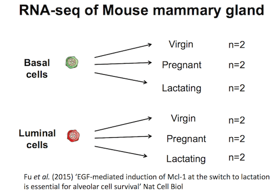
Mouse mammary gland dataset
The information for this tutorial comes from a Nature Jail cell Biology paper by Fu et al. 2015. Both the raw data (sequence reads) and processed data (counts) tin can be downloaded from Gene Expression Autobus database (GEO) under accession number GSE60450.
This study examined the expression profiles of basal and luminal cells in the mammary gland of virgin, pregnant and lactating mice. Vi groups are present, with i for each combination of cell blazon and mouse status. Note that two biological replicates are used here, ii independent sorts of cells from the mammary glands of virgin, pregnant or lactating mice, withal three replicates is normally recommended as a minimum requirement for RNA-seq.
This is a Milky way tutorial based on material from the COMBINE R RNAseq workshop, first taught here.
Figure ane: Tutorial Dataset
Agenda
In this tutorial, we will cover:
Preparing the reads
Import information from URLs
Raw reads QC
Trim reads
Trimmed reads QC
Mapping
Map reads to reference genome
Counting
Count reads mapped to genes
Create count matrix
Generating a QC summary report
Strandness
Duplicate reads
Reads mapped to chromosomes
Gene body coverage (5'-3')
Read distribution across features (exons, introns, intergenic..)
Preparing the reads
Import data from URLs
Read sequences are usually stored in compressed (gzipped) FASTQ files. Before the differential expression analysis can proceed, these reads must be aligned to the reference genome and counted into annotated genes. Mappingreads to the genome is a very important task, and many different aligners are bachelor, such every bit HISAT2 (Kim et al. 2015), STAR (Dobin et al. 2013) and Subread (Liao et al. 2013). Nearly mapping tasks require larger computers than an boilerplate laptop, and so usually read mapping is done on a server in a linux-like environs, requiring some programming knowledge. However, Galaxy enables you to practice this mapping without needing to know programming and if you don't take access to a server y'all can endeavor to employ 1 of the publically available Galaxies due east.g. usegalaxy.org, usegalaxy.eu, employgalaxy.org.au.
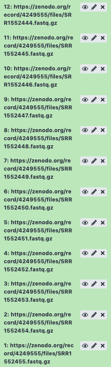
The raw reads used in this tutorial were obtained from SRA from the link in GEO for the the mouse mammary gland dataset (eastward.g ftp://ftp-trace.ncbi.nlm.nih.gov/sra/sra-instant/reads/ByStudy/sra/SRP%2FSRP045%2FSRP045534). For the purpose of this tutorial nosotros are going to be working with a small office of the FASTQ files. We are only going to exist mapping grand reads from each sample to enable running through all the steps quickly. If working with your own data yous would use the full data and some results for the total mouse dataset volition exist shown for comparison. The small FASTQ files are available in Zenodo and the links to the FASTQ files are provided beneath.
If you are sequencing your own data, the sequencing facility volition near always provide compressed FASTQ files which yous can upload into Galaxy. For sequence data available through URLs, The Galaxy Rule-based Uploader can exist used to import the files. It is much quicker than downloading FASTQs to your estimator and uploading into Galaxy and also enables importing as a Collection. When you take more than a few files, using Milky way Collections helps proceed the datasets organised and tidy in the history. Collections also make it easier to maintain the sample names through tools and workflows. If you are not familiar with collections, you can take a wait at the Milky way Collections tutorial for more than details. The screenshots below prove a comparison of what the FASTQ datasets for this tutorial would wait like in the history if nosotros imported them as datasets versus every bit a collection with the Rule-based Uploader.
Datasets
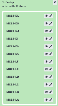
Collection
details Collections and sample names
Collections tin likewise help to maintain the original sample names on the files throughout the tools used. The screenshots below show what we would meet in i of the MultiQC reports that we volition generate if we used datasets versus a collection.
Datasets
Collection
The data nosotros need to import the samples for this tutorial (sample ID, Group, and link to the FASTQ file (URL) are in the grey box below.
In lodge to get these files into Galaxy, nosotros will desire to exercise a few things:
Strip the header out of the sample information (information technology doesn't contain a URL Galaxy can download).
Define the file Identifier column (SampleID).
Define the URL column (URL) (this is the location Galaxy tin download the data from).
hands_on Hands-on: Data upload
Create a new history for this tutorial e.g. RNA-seq reads to counts
Tip: Creating a new history
Click the new-history icon at the top of the history panel.
If the new-history is missing:
Click on the galaxy-gear icon (History options) on the top of the history console
Select the option Create New from the carte
Tip: Renaming a history
Click on Unnamed history (or the current name of the history) (Click to rename history) at the summit of your history panel
Blazon the new name
Press Enter
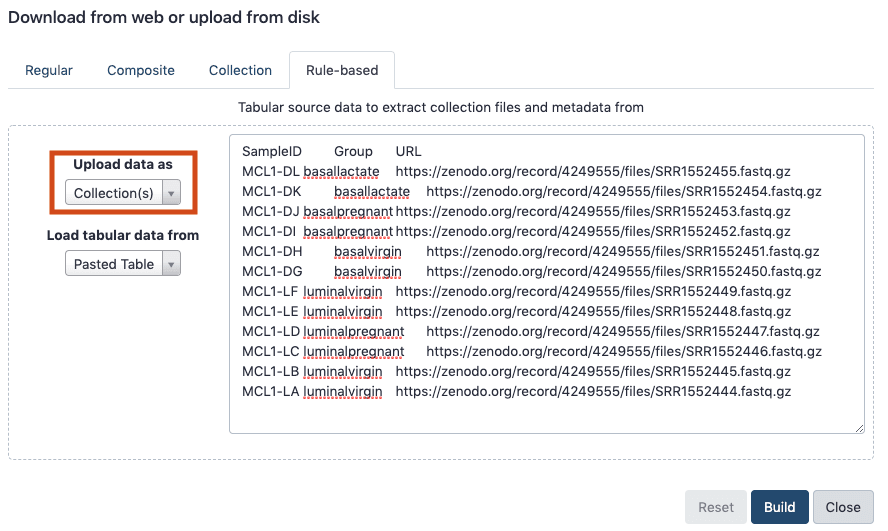
Import the files from Zenodo using Milky way'south Rule-based Uploader.
Open the Galaxy Upload Managing director
Click the tab Rule-based
"Upload data as": Collection(southward)
"Load tabular data from": Pasted Table
Paste the tabular array from the grey box above. (Yous should now run across below)
Click Build
Figure 2: Rule-based Uploader
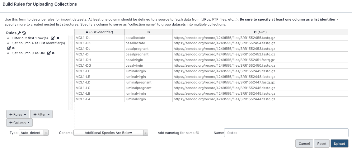
In the rules editor that pops up:
Remove the header. From the Filter menu select First or Last N Rows
"Filter which rows?": offset
"Filter how many rows?": ane
Click Apply
Define the Identifier and URL columns. From the Rules card select Add / Modify Column Definitions
Click Add together Definition push button and select List Identifier(south)
"List Identifier(southward)": A
Click Add Definition push button again and select URL instead
"URL": C
Click Utilize, and you should see your new column definitions listed
Proper noun the collection. For "Name" enter: fastqs(Y'all should at present see below)
Click Upload
Figure three: Rules Editor
You should see a collection (list) called fastqs in your history containing all 12 FASTQ files.
If your data is not accessible past URL, for example, if your FASTQ files are located on your laptop and are not likewise large, you tin can upload into a collection as below. If they are big you could use FTP. Y'all can take a expect at the Getting information into Galaxy slides for more than data.
tip Tip: Upload local files into a collection
Open up the Galaxy Upload Managing director
Click the tab Collection
Click Cull Local Files and locate the files you want to upload
"Drove Type": List
In the pop up that appears:
"Proper noun": fastqs
Click Create listing
If your FASTQ files are located in Shared Data, you can import them into your history every bit a drove as below.
tip Tip: Import files from Shared Data into a collection
In the Menu at the height go to Shared Information > Data Libraries
Locate your FASTQ files
Tick the checkboxes to select the files
From the To History menu select as a Collection
In the popular up that appears:
"Which datasets?": current selection
"Collection type": List
"Select history": select your History
Click Proceed
In the pop up that appears:
"Name": fastqs
Click Create listing
Have a wait at ane of the FASTQ files to see what it contains.
hands_on Hands-on: Take a look at FASTQ format
Click on the drove name (fastqs)
Click on the galaxy-centre (eye) icon of one of the FASTQ files to have a look at what information technology contains
details FASTQ format
If you are non familiar with FASTQ format, see the Quality Command tutorial
Raw reads QC
During sequencing, errors are introduced, such equally incorrect nucleotides beingness called. These are due to the technical limitations of each sequencing platform. Sequencing errors might bias the analysis and can lead to a misinterpretation of the information. Every base of operations sequence gets a quality score from the sequencer and this information is nowadays in the FASTQ file. A quality score of 30 corresponds to a 1 in m chance of an incorrect base call (a quality score of 10 is a ane in 10 gamble of an incorrect base telephone call). To look at the overall distribution of quality scores across the reads, we tin use FastQC.
Sequence quality control is therefore an essential first stride in your analysis. We volition use similar tools as described in the "Quality control" tutorial: FastQC and Cutadapt (Marcel 2011).
hands_on Hands-on: Check raw reads with FastQC
FastQCtool with the following parameters:
param-collection"Short read data from your current history": fastqs (Input dataset collection)
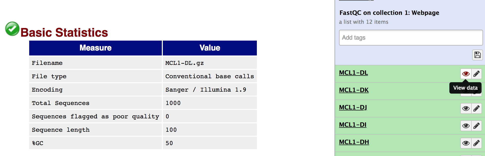
Audit the Webpage output of FastQCtool for the MCL1-DL sample by clicking on the galaxy-eye (eye) icon
Tip: Selecting a datast collection as input
Click on param-collectionDataset collection in forepart of the input parameter you desire to supply the collection to.
Select the drove you desire to utilise from the list
question Questions
What is the read length?
What base quality score encoding is used?
solution Solution
The read length is 100 bp.
Sanger quality score encoding is used. This information can be seen at the height of the FastQC Webpage as below.
Effigy 4: FastQC Webpage
The FastQC report contains a lot of data and nosotros can expect at the report for each sample. Yet, that is quite a few reports, 12 for this dataset. If you had more samples it could be a lot more. Luckily, there is a very useful tool called MultiQC (Ewels et al. 2016) that can summarise QC data for multiple samples into a single report. We'll generate a few MultiQC outputs in this tutorial then we'll add name tags so we tin can differentiate them.
hands_on Hands-on: Amass FastQC reports with MultiQC
MultiQCtool with the following parameters to amass the FastQC reports
In "Results"
param-select"Which tool was used generate logs?": FastQC
In "FastQC output"
param-select"Type of FastQC output?": Raw data
param-collection"FastQC output": RawData files (output of FastQCtool on trimmed reads)
Add a tag #fastqc-raw to the Webpage output from MultiQC and inspect the webpage
Tip: Adding a tag
Click on the dataset
Click on milky way-tagsEdit dataset tags
Add a tag starting with #
Tags starting with # will be automatically propagated to the outputs of tools using this dataset.
Cheque that the tag is appearing beneath the dataset name
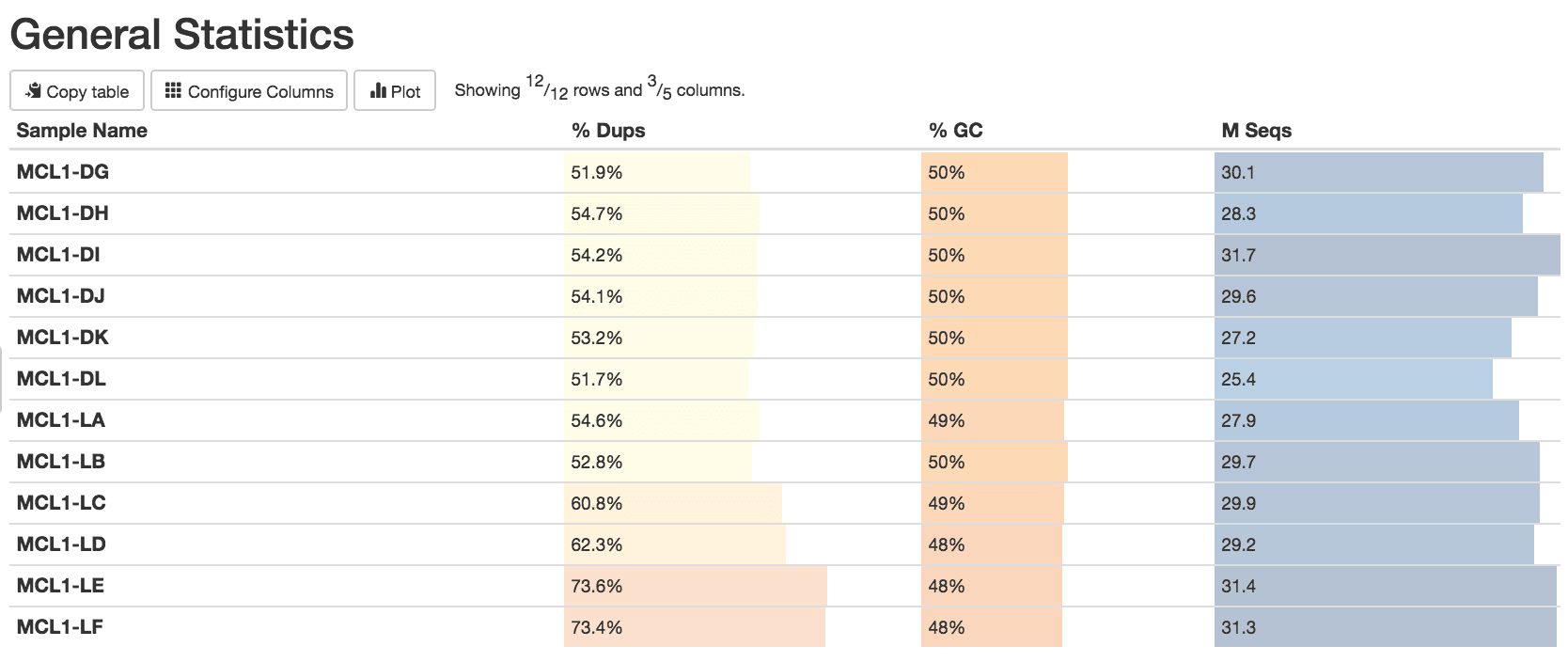
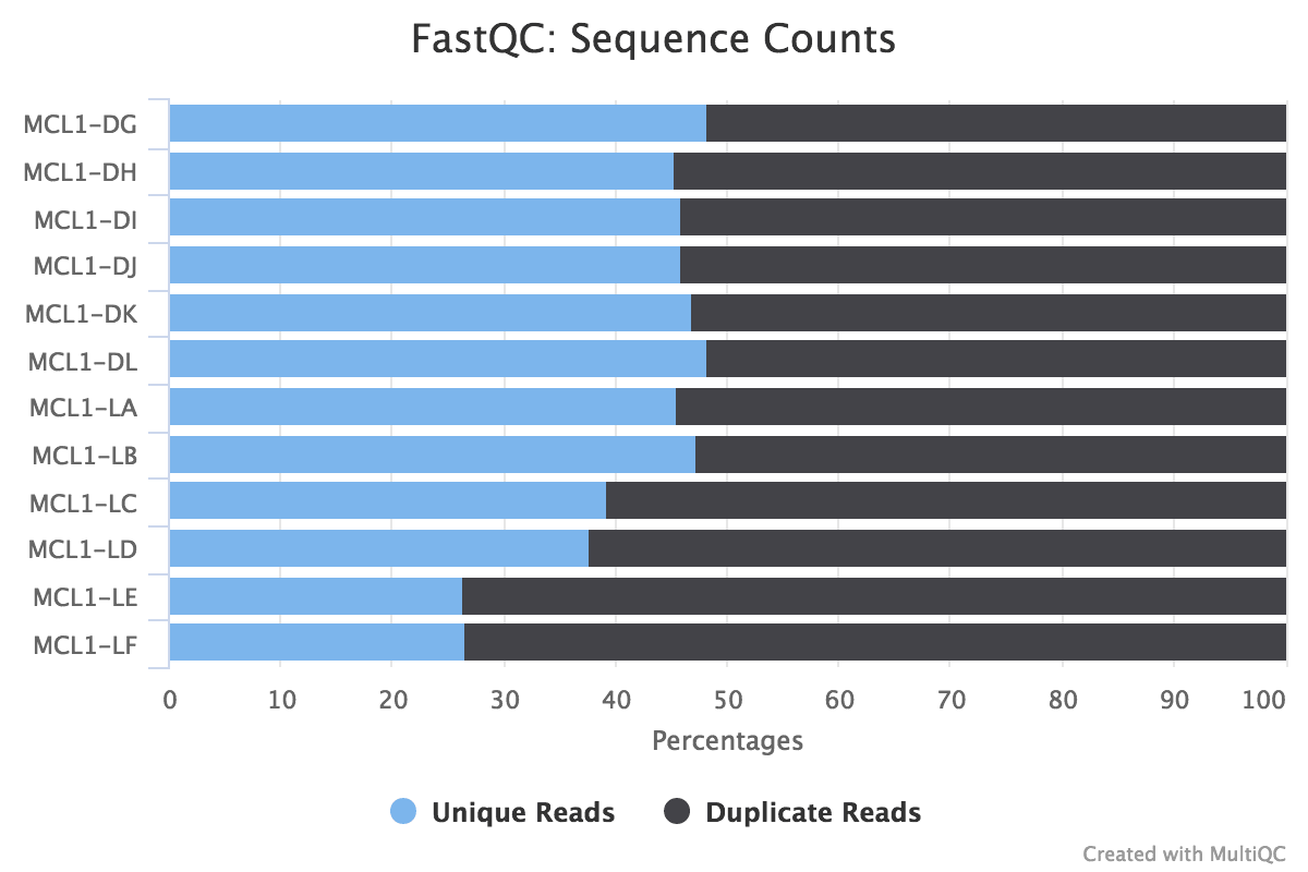
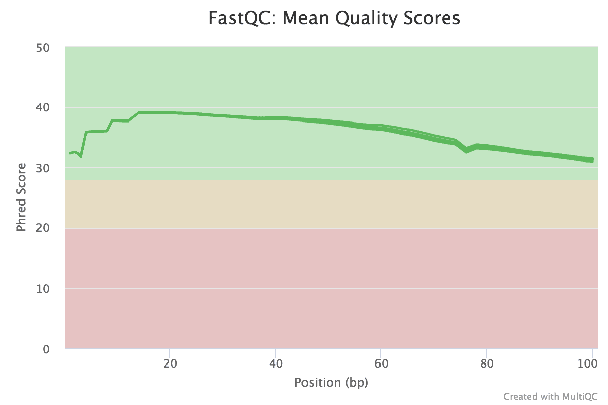
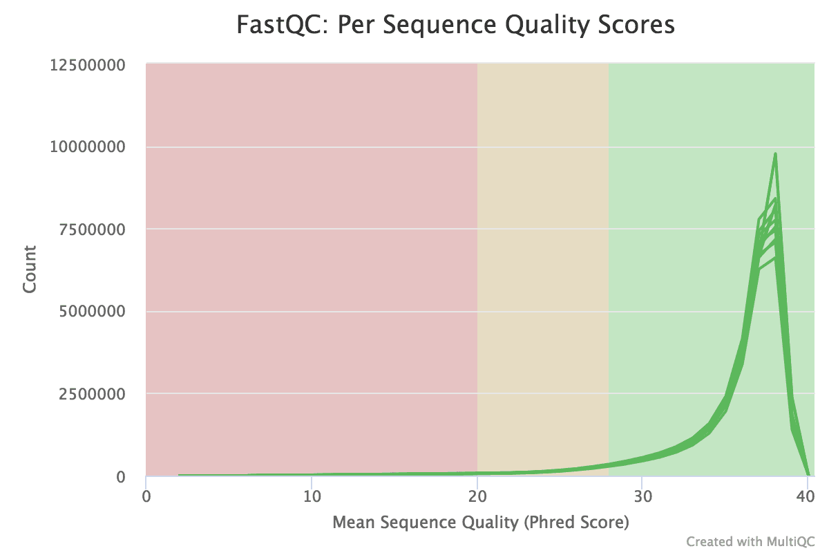
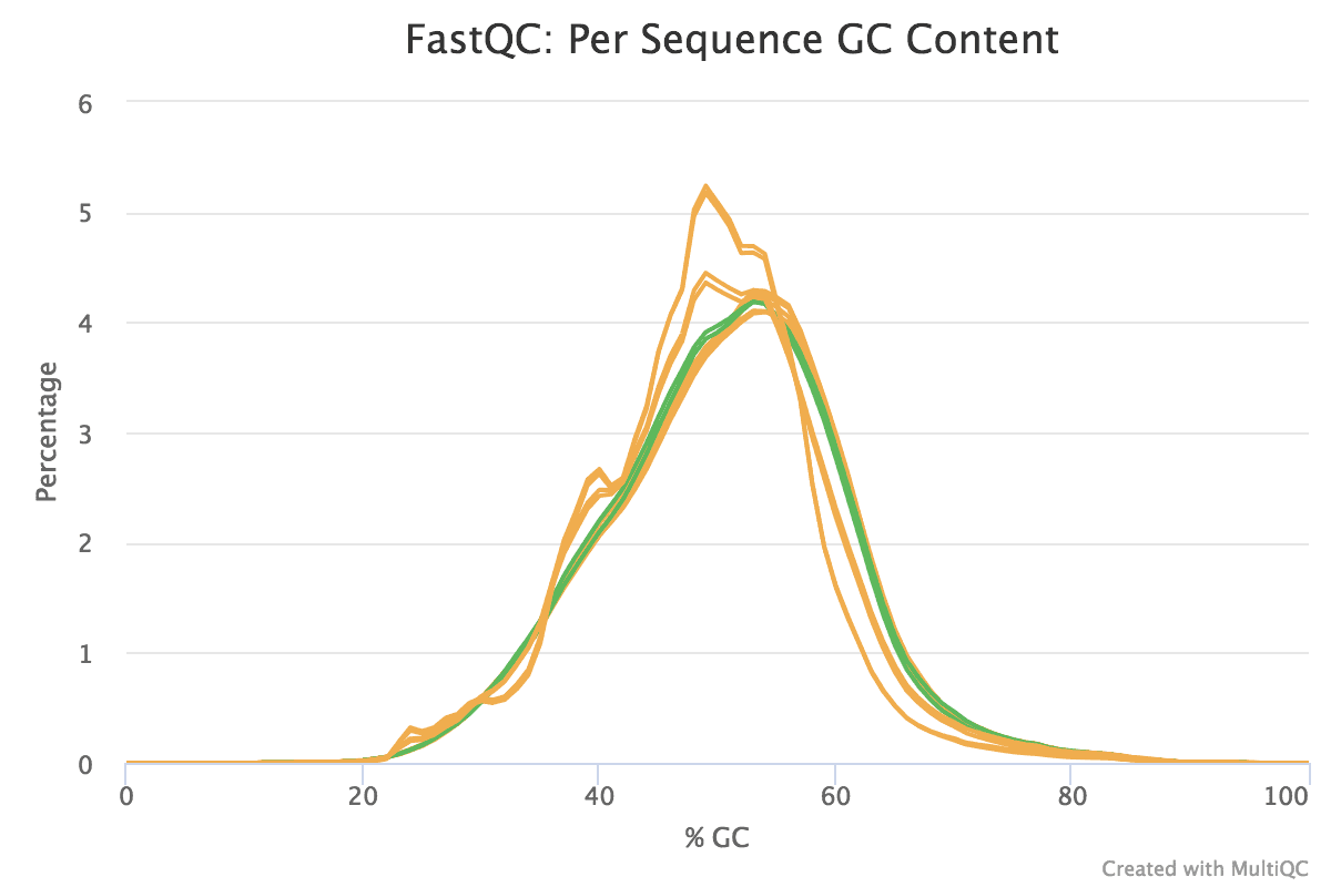
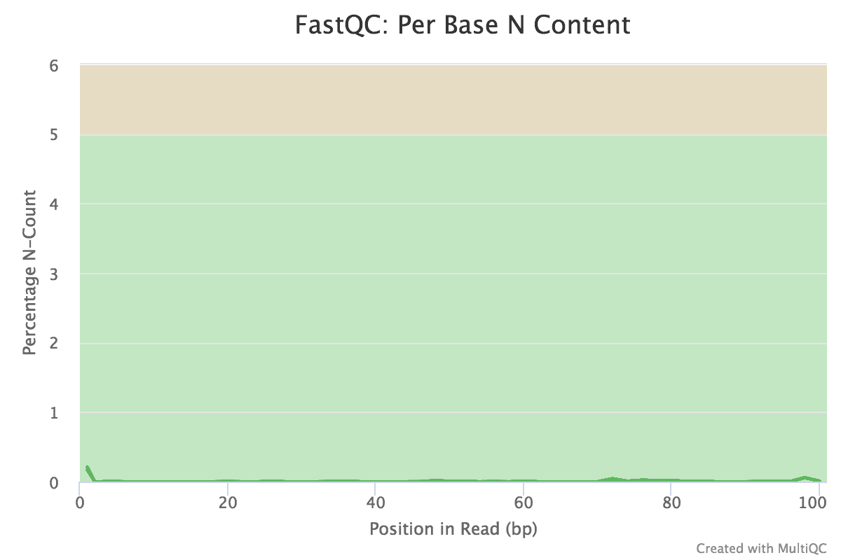
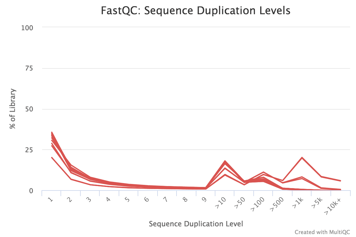
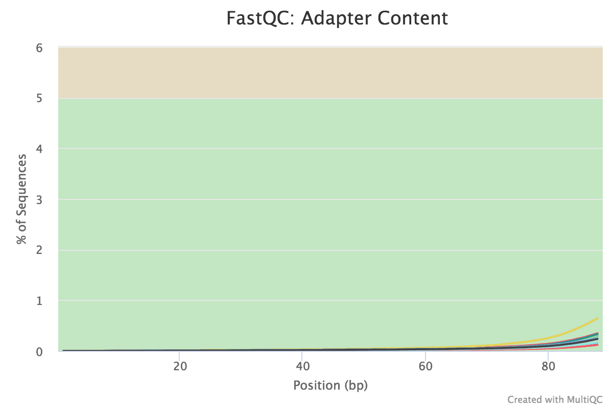
Note that these are the results for simply m reads. The FastQC results for the total dataset are shown below. The 1000 reads are the beginning reads from the FASTQ files, and the commencement reads usually originate from the flowcell edges, so nosotros can expect that they may have lower quality and the patterns may be a fleck dissimilar from the distribution in the total dataset.
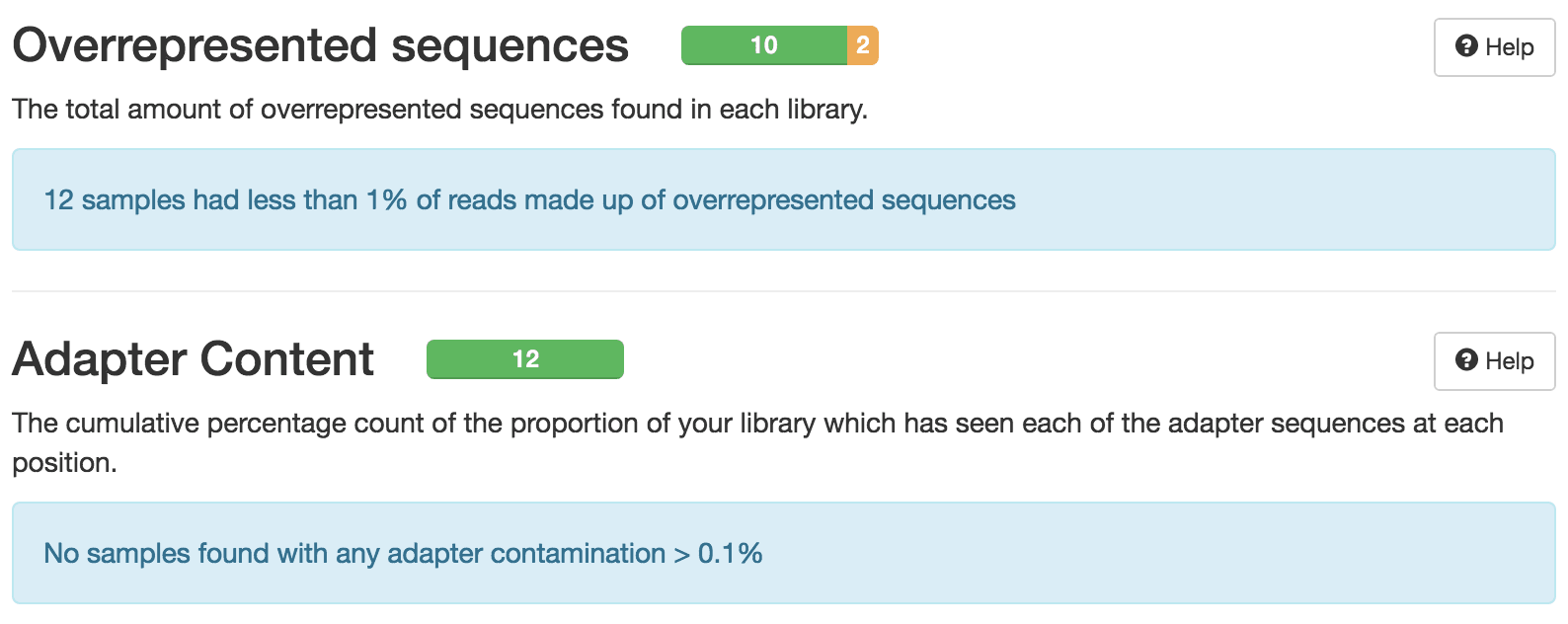
You should see that most of the plots in the small FASTQs expect like to the full dataset. However, in the minor FASTQs, there is less duplication, some Ns in the reads and some overrepresented sequences.
Figure v: General StatisticsEffigy 6: Sequence CountsFigure 7: Sequence QualityFigure viii: Per Sequence Quality ScoresEffigy 9: Per Sequence GC ContentFigure ten: Per base N contentFigure 11: Sequence Duplication LevelsFigure 12: Adapter Content
Encounter the Quality Control tutorial for more than information on FastQC plots.
question Questions
What practice you think of the overall quality of the sequences?
solution Solution
Overall, the samples look pretty skilful. The primary things to note here are:
The base of operations quality is loftier in all samples.
Some Illumina adapter has been detected.
Some duplication in RNA-seq can be normal due to the presence of highly expressed genes. However, for some reason MCL1-LE and MCL1-LF have higher numbers of duplicates detected than the other samples.
We will utilise Cutadapt to trim the reads to remove the Illumina adapter and any low quality bases at the ends (quality score < twenty). We will discard whatever sequences that are too short (< 20bp) after trimming. We volition also output the Cutadapt report for summarising with MultiQC.
The Cutadapt tool Assist section provides the sequence we can utilize to trim this standard Illumina adapter AGATCGGAAGAGCACACGTCTGAACTCCAGTCAC, as given on the Cutadapt website. For trimming paired-end information see the Cutadapt Help section. Other Illumina adapter sequences (e.1000. Nextera) can exist found at the Illumina website. Note that Cutadapt requires at least three bases to friction match betwixt adapter and read to reduce the number of falsely trimmed bases, which can be changed in the Cutadapt options if desired.
Trim reads
hands_on Easily-on: Trim reads with Cutadapt
Cutadapttool with the following parameters:
param-select"Single-terminate or Paired-end reads?": Single-end
We tin can have a look at the reads again now that they've been trimmed.
Trimmed reads QC
hands_on Hands-on: QC of trimmed reads with FastQC
FastQCtool with the post-obit parameters:
param-drove"Short read data from your electric current history": RawData (output of Cutadapttool)
MultiQCtool with the post-obit parameters to aggregate the FastQC reports
In "Results"
param-select"Which tool was used generate logs?": FastQC
In "FastQC output"
param-select"Type of FastQC output?": Raw information
param-drove"FastQC output": RawData files (output of FastQCtool)
Add a tag #fastqc-trimmed to the Webpage output from MultiQC and audit the webpage
The MultiQC plot beneath shows the upshot from the full dataset for comparison.
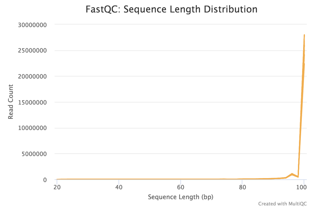
Figure thirteen: Adapter Content postal service-trimmingFigure fourteen: Sequence Length post-trimming
After trimming we can see that:
No adapter is detected now.
The reads are no longer withal length, we at present have sequences of different lengths detected.
Mapping
Now that we accept prepared our reads, we can align the reads for our 12 samples. There is an existing reference genome for mouse and we will map the reads to that. The current most widely used version of the mouse reference genome is mm10/GRCm38 (although note that there is a new version mm39 released June 2020). Here we volition utilise HISAT2 to align the reads. HISAT2 is the descendent of TopHat, one of the showtime widely-used aligners, just alternative mappers could exist used, such as STAR. See the RNA-seq ref-based tutorial for more information on RNA-seq mappers. In that location are often numerous mapping parameters that we can specify, but usually the default mapping parameters are fine. However, library type (paired-cease vs unmarried-cease) and library strandness (stranded vs unstranded) require some different settings when mapping and counting, so they are two important pieces of information to know nigh samples. The mouse data comprises unstranded, unmarried-stop reads then nosotros will specify that where necessary. HISAT2 tin output a mapping summary file that tells what proportion of reads mapped to the reference genome. Summary files for multiple samples can exist summarised with MultiQC. As we're merely using a subset of 1000 reads per sample, adjustment should just have a minute or so. To run the full samples from this dataset would have longer.
Map reads to reference genome
hands_on Easily-on: Map reads to reference with HISAT2
HISAT2tool with the following parameters:
param-select"Source for the reference genome": Use a built-in genome
param-select"Select a reference genome": mm10
param-select"Is this a single or paired library?": Single-end
param-collection"FASTA/Q file": Read one Output (output of Cutadapttool)
In "Summary Options":
param-check"Output alignment summary in a more machine-friendly style.": Yes
param-check"Print alignment summary to a file.": Yes
MultiQCtool with the following parameters to aggregate the HISAT2 summary files
In "Results"
param-select"Which tool was used generate logs?": HISAT2
param-collection"Output of HISAT2": Mapping summary (output of HISAT2tool)
Add a tag #hisat to the Webpage output from MultiQC and inspect the webpage
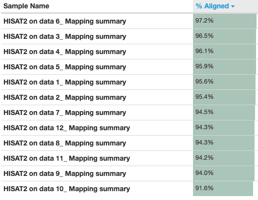
The MultiQC plot beneath shows the effect from the full dataset for comparison.
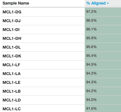
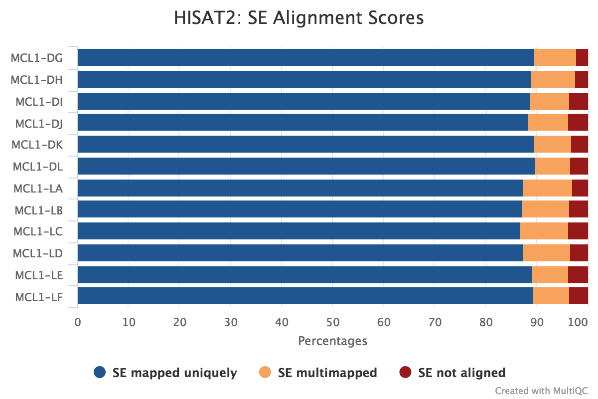
Figure fifteen: HISAT2 mapping
An important metric to cheque is the percentage of reads mapped to the reference genome. A low percent tin betoken problems with the data or assay. Over 90% of reads have mapped in all samples, which is a good mapping charge per unit, and the vast majority of reads have mapped uniquely, they haven't mapped to multiple locations in the reference genome.
It is besides good practice to visualise the read alignments in the BAM file, for example using IGV, see the RNA-seq ref-based tutorial.
HISAT2 generates a BAM file with mapped reads.
A BAM (Binary Alignment Map) file is a compressed binary file storing the read sequences, whether they have been aligned to a reference sequence (e.g. a chromosome), and if so, the position on the reference sequence at which they have been aligned.
hands_on Easily-on: Audit a BAM/SAM file
Inspect the param-file output of HISAT2tool
A BAM file (or a SAM file, the non-compressed version) consists of:
A header section (the lines starting with @) containing metadata particularly the chromosome names and lengths (lines starting with the @SQ symbol)
An alignment department consisting of a tabular array with eleven mandatory fields, as well as a variable number of optional fields:
Col
Field
Type
Brief Description
1
QNAME
String
Query template NAME
ii
FLAG
Integer
Bitwise FLAG
3
RNAME
String
References sequence NAME
iv
POS
Integer
ane- based leftmost mapping POSition
5
MAPQ
Integer
MAPping Quality
6
CIGAR
Cord
CIGAR String
7
RNEXT
String
Ref. name of the mate/next read
8
PNEXT
Integer
Position of the mate/next read
nine
TLEN
Integer
Observed Template LENgth
10
SEQ
Cord
Segment SEQuence
eleven
QUAL
String
ASCII of Phred-scaled base QUALity+33
question Questions
Which information do you discover in a SAM/BAM file?
What is the additional information compared to a FASTQ file?
solution Solution
Sequences and quality information, like a FASTQ
Mapping information, Location of the read on the chromosome, Mapping quality, etc
tip Tip: Downloading a collection
To download a collection of datasets (east.one thousand. the collection of BAM files) click on the floppy disk icon within the drove. This volition download a tar file containing all the datasets in the drove. Note that for BAM files the .bai indexes (required for IGV) will be included automatically in the download.
Counting
The alignment produces a set of BAM files, where each file contains the read alignments for each sample. In the BAM file, at that place is a chromosomal location for every read that mapped. Now that we have figured out where each read comes from in the genome, nosotros demand to summarise the data across genes or exons. The mapped reads tin be counted across mouse genes by using a tool called featureCounts (Liao et al. 2013). featureCounts requires gene annotation specifying the genomic offset and stop position of each exon of each gene. For convenience, featureCounts contains built-in annotation for mouse (mm10, mm9) and homo (hg38, hg19) genome assemblies, where exon intervals are defined from the NCBI RefSeq annotation of the reference genome. Reads that map to exons of genes are added together to obtain the count for each gene, with some care taken with reads that bridge exon-exon boundaries. The output is a count for each Entrez Cistron ID, which are numbers such as 100008567. For other species, users volition need to read in a data frame in GTF format to ascertain the genes and exons. Users can too specify a custom annotation file in SAF format. Encounter the tool help in Galaxy, which has an example of what an SAF file should like like, or the Rsubread users guide for more information.
Count reads mapped to genes
hands_on Hands-on: Count reads mapped to genes with featureCounts
featureCountstool with the following parameters:
param-drove"Alignment file": aligned reads (BAM) (output of HISAT2tool)
param-select"Factor annotation file": featureCounts born
param-select"Select built-in genome": mm10
MultiQCtool with the following parameters:
param-select"Which tool was used generate logs?": featureCounts
param-collection"Output of FeatureCounts": featureCounts summary (output of featureCountstool)
Add a tag #featurecounts to the Webpage output from MultiQC and inspect the webpage
The MultiQC plot below shows the result from the full dataset for comparison.
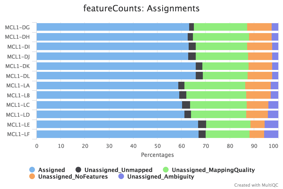
Figure xvi: featureCounts assignments
question Questions
What % reads are assigned to exons?
solution Solution
~threescore-seventy% of reads are assigned to exons. This is a adequately typical number for RNA-seq.
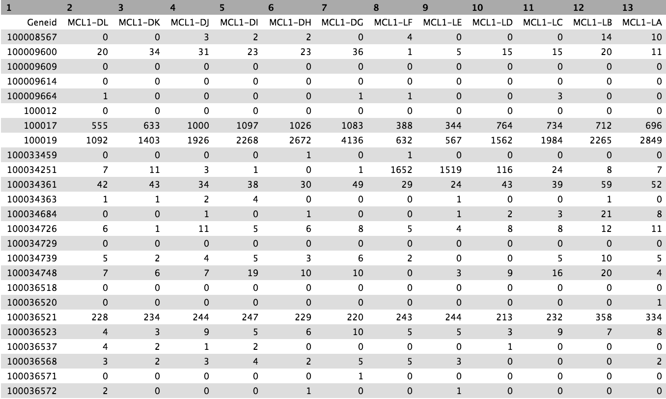
The counts for the samples are output as tabular files. Have a look at one. The numbers in the showtime cavalcade of the counts file correspond the Entrez gene identifiers for each gene, while the second column contains the counts for each gene for the sample.
Create count matrix
The counts files are currently in the format of one file per sample. Withal, it is ofttimes convenient to have a count matrix. A count matrix is a unmarried table containing the counts for all samples, with the genes in rows and the samples in columns. The counts files are all within a collection so we tin can employ the Milky wayColumn Join on multiple datasets tool to easily create a count matrix from the single counts files.
hands_on Hands-on: Create count matrix with Cavalcade Join on multiple datasets
Column Join on multiple datasetsTool: toolshed.g2.bx.psu.edu/repos/iuc/collection_column_join/collection_column_join/0.0.3 with the post-obit parameters:
param-collection"Tabular files": Counts (output of featureCountstool)
param-text"Identifier column": 1
param-text"Number of header lines in each input file": i
param-check"Add column name to header": No
Accept a await at the output. The tutorial uses a pocket-sized subset of the data ~ 1000 reads per sample to save on processing time. Most rows in that matrix will contain all zeros, at that place will exist ~600 non-zilch rows. The output for the full dataset is shown beneath.
Figure 17: Count matrix
Now information technology is easier to see the counts for a gene across all samples. The accompanying tutorial, RNA-seq counts to genes, shows how gene data (symbols etc) tin can be added to a count matrix.
Generating a QC summary study
There are several additional QCs we tin perform to better sympathize the data, to see if information technology's proficient quality. These tin can also aid determine if changes could be made in the lab to meliorate the quality of hereafter datasets.
Nosotros'll employ a prepared workflow to run the kickoff few of the QCs beneath. This will also demonstrate how y'all can make apply of Galaxy workflows to easily run and reuse multiple assay steps. The workflow will run the first three tools: Infer Experiment, MarkDuplicates and IdxStats and generate a MultiQC report. You can and so edit the workflow if yous'd similar to add other steps.
hands_on Hands-on: Run QC written report workflow
Import the workflow into Galaxy
Copy the URL (e.k. via right-click) of this workflow or download it to your computer.
Import the workflow into Milky way
Tip: Importing a workflow
Click on Workflow on the height menu bar of Galaxy. You will see a listing of all your workflows.
Click on the upload icon galaxy-upload at the peak-right of the screen
Provide your workflow
Selection ane: Paste the URL of the workflow into the box labelled "Archived Workflow URL"
Option 2: Upload the workflow file in the box labelled "Archived Workflow File"
Open up the Milky way Upload Manager (galaxy-upload on the top-right of the tool panel)
Select Paste/Fetch Data
Paste the link into the text field
Press Start
Close the window
Run Workflow QC Reportworkflow using the post-obit parameters:
"Send results to a new history": No
param-file"1: Reference genes": the imported RefSeq BED file
param-collection"2: BAM files": aligned reads (BAM) (output of HISAT2tool)
Tip: Running a workflow
Click on Workflow on the acme carte du jour bar of Galaxy. You lot will run into a list of all your workflows.
Click on the workflow-run (Run workflow) button next to your workflow
Configure the workflow every bit needed
Click the Run Workflow push button at the superlative-right of the screen
Yous may have to refresh your history to come across the queued jobs
Inspect the Webpage output from MultiQC
You do not demand to run the hands-on steps beneath. They are just to show how you could run the tools individually and what parameters to set.
Strandness
As far as we know this data is unstranded, but as a sanity check you tin can check the strandness. You can utilize RSeQC Infer Experiment tool to "approximate" the strandness, equally explained in the RNA-seq ref-based tutorial. This is done through comparing the "strandness of reads" with the "strandness of transcripts". For this tool, and many of the other RSeQC (Wang et al. 2012) tools, a reference bed file of genes (reference genes) is required. RSeQC provides some reference BED files for model organisms. You can import the RSeQC mm10 RefSeq BED file from the link https://sourceforge.internet/projects/rseqc/files/BED/Mouse_Mus_musculus/mm10_RefSeq.bed.gz/download (and rename to reference genes) or import a file from Shared data if provided. Alternatively, you can provide your own BED file of reference genes, for instance from UCSC (see the Peaks to Genes tutorial. Or the Convert GTF to BED12 tool can be used to convert a GTF into a BED file.
hands_on Hands-on: Check strandness with Infer Experiment
Infer Experimenttool with the following parameters:
param-collection"Input .bam file": aligned reads (BAM) (output of HISAT2tool)
param-file"Reference gene model": reference genes (Reference BED file)
MultiQCtool with the following parameters:
In "i: Results":
param-select"Which tool was used generate logs?": RSeQC
param-select"Type of RSeQC output?": infer_experiment
param-collection"RSeQC infer_experiment output": Infer Experiment output (output of Infer Experimenttool)
Inspect the Webpage output from MultiQC
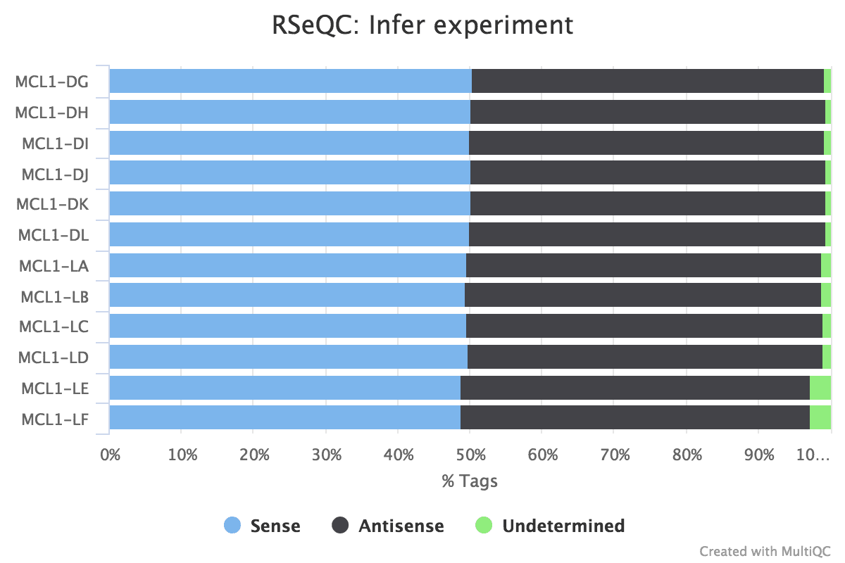
The MultiQC plot below shows the result from the full dataset for comparison.
Figure 18: Infer Experiment
question Questions
Practice you think the data is stranded or unstranded?
solution Solution
It is unstranded every bit approximately equal numbers of reads have aligned to the sense and antisense strands.
Indistinguishable reads
Duplicate reads are usually kept in RNA-seq differential expression analysis as they can come up from highly-expressed genes but it is still a good metric to cheque. A high percentage of duplicates can indicate a problem with the sample, for example, PCR amplification of a depression complexity library (not many transcripts) due to non enough RNA used as input. FastQC gives united states of america an thought of duplicates in the reads earlier mapping (note that it just takes a sample of the data). Nosotros can assess the numbers of duplicates in all mapped reads using the Picard MarkDuplicates tool. Picard considers duplicates to exist reads that map to the aforementioned location, based on the get-go position of where the read maps. In general, we consider normal to obtain up to 50% of duplication.
hands_on Hands-on: Bank check indistinguishable reads with MarkDuplicates
MarkDuplicatestool with the following parameters:
param-drove"Select SAM/BAM dataset or dataset collection": aligned reads (BAM) (output of HISAT2tool)
MultiQCtool with the following parameters:
In "1: Results":
param-select"Which tool was used generate logs?": Picard
param-select"Type of Picard output?": Markdups
param-collection"Picard output": MarkDuplicate metrics (output of MarkDuplicatestool)
Audit the Webpage output from MultiQC
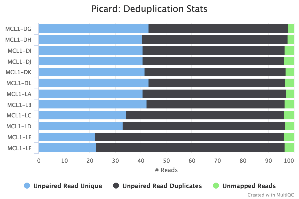
The MultiQC plot below shows the upshot from the full dataset for comparison.
Figure 19: MarkDups metrics
question Questions
Which ii samples have the most duplicates detected?
solution Solution
MCL1-LE and MCL1-LF have the highest number of duplicates in mapped reads compared to the other samples, similar to what nosotros saw in the raw reads with FastQC.
Reads mapped to chromosomes
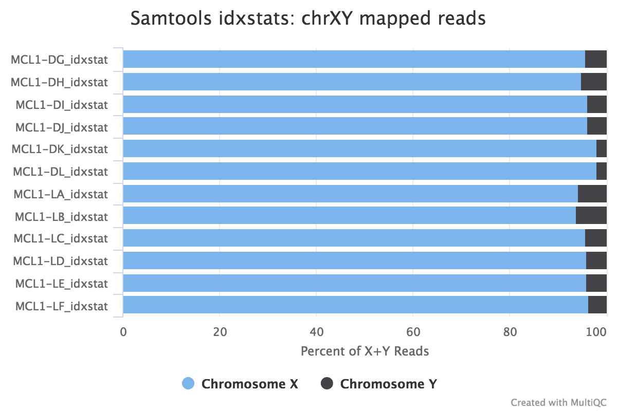
You tin cheque the numbers of reads mapped to each chromosome with the Samtools IdxStats tool. This can aid assess the sample quality, for example, if there is an excess of mitochondrial contagion. It could as well help to check the sex of the sample through the numbers of readsmapping to 10/Y or to run into if any chromosomes have highly expressed genes.
hands_on Hands-on: Count readsmapping to each chromosome with IdxStats
IdxStatstool with the following parameters:
param-collection"BAM file": aligned reads (BAM) (output of HISAT2tool)
MultiQCtool with the following parameters:
In "ane: Results":
param-select"Which tool was used generate logs?": Samtools
param-select"Type of Samtools output?": idxstats
param-collection"Samtools idxstats output": IdxStats output (output of IdxStatstool)
Inspect the Webpage output from MultiQC
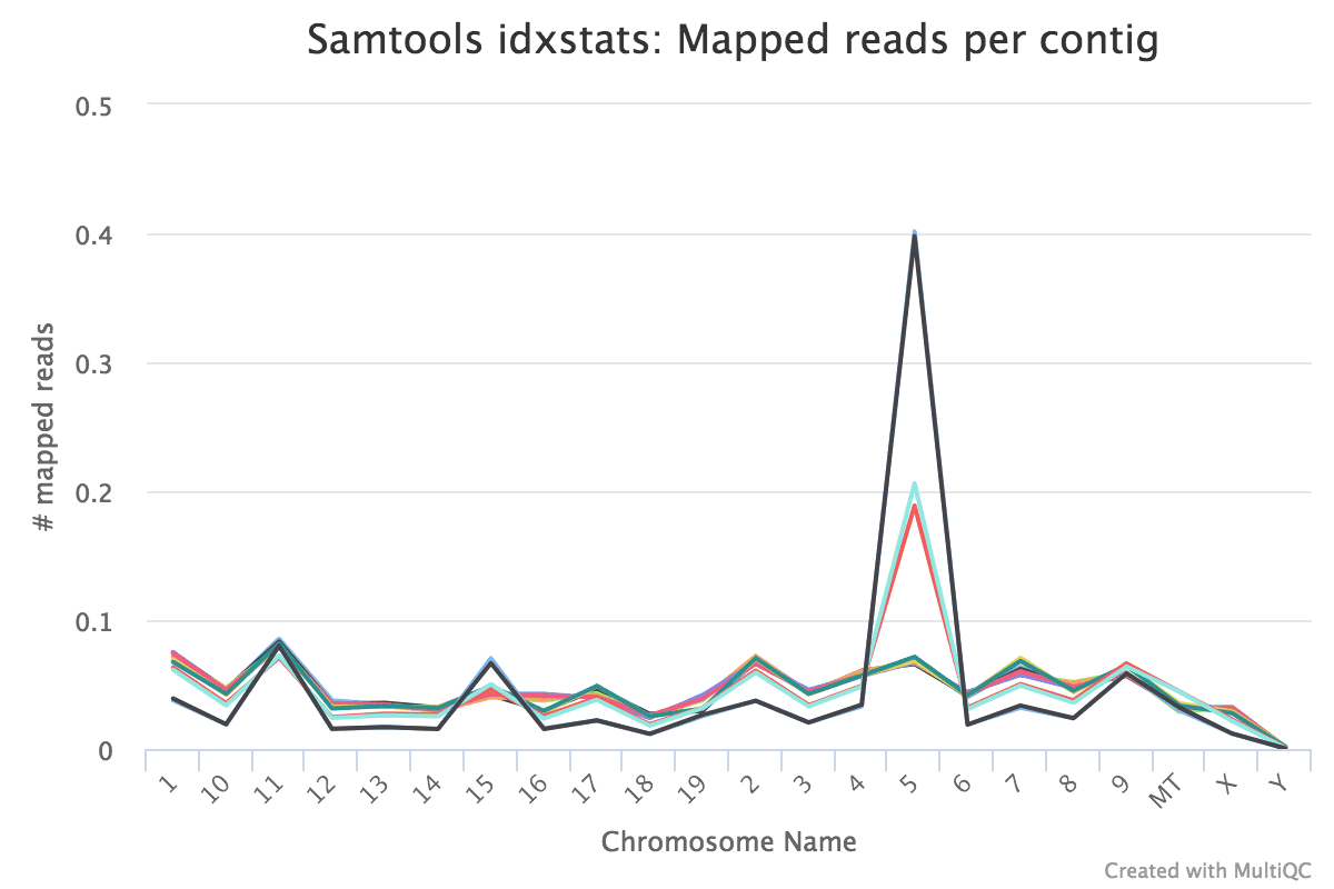
The MultiQC plot below shows the result from the total dataset for comparison.
Figure 20: IdxStats Chromosome MappingsFigure 21: IdxStats X/Y Mappingdue south
question Questions
What do you retrieve of the chromosome mappings?
Are the samples male or female? (If a sample is not in the XY plot information technology means no reads mapped to Y)
solution Solution
Some of the samples have very high mapping on chromosome 5. What is going on in that location?
The samples appear to be all female equally at that place are few readsmapping to the Y chromosome. As this is a experiment studying virgin, significant and lactating mice if we saw large numbers of readsmapping to the Y chromosome in a sample it would be unexpected and a probable cause for business organization.
Cistron trunk coverage (v'-3')
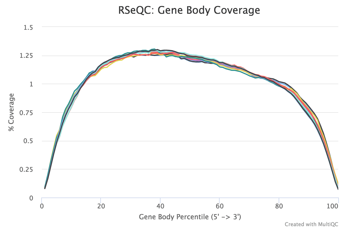
The coverage of reads along gene bodies tin be assessed to check if there is any bias in coverage. For example, a bias towards the 3' end of genes could betoken degradation of the RNA. Alternatively, a 3' bias could betoken that the data is from a 3' assay (e.g. oligodT-primed, 3'RNA-seq). You can use the RSeQC Factor Torso Coverage (BAM) tool to assess cistron body coverage in the BAM files.
hands_on Hands-on: Check coverage of genes with Gene Torso Coverage (BAM)
Cistron Body Coverage (BAM)tool with the following parameters:
"Run each sample separately, or combine mutiple samples into 1 plot": Run each sample separately
param-collection"Input .bam file": aligned reads (BAM) (output of HISAT2tool)
param-select"Which tool was used generate logs?": RSeQC
param-select"Type of RSeQC output?": gene_body_coverage
param-collection"RSeQC gene_body_coverage output": Gene Body Coverage (BAM) (text) (output of Gene Body Coverage ( BAM)tool)
Inspect the Webpage output from MultiQC
The MultiQC plot below shows the effect from the full dataset for comparing.
Effigy 22: Gene Trunk Coverage
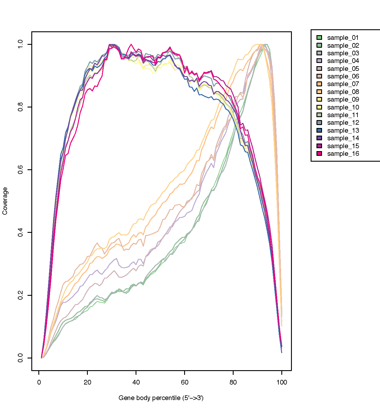
The plot beneath from the RSeQC website shows what samples with three'biased coverage would expect like.
Figure 23: Gene Body Coverage comparison
question Questions
What exercise you think of the coverage across gene bodies in these samples?
solution Solution
It looks skillful. This plot looks a chip noisy in the small FASTQs just information technology still shows there's pretty even coverage from 5' to iii' ends with no obvious bias in all the samples.
Read distribution across features (exons, introns, intergenic..)
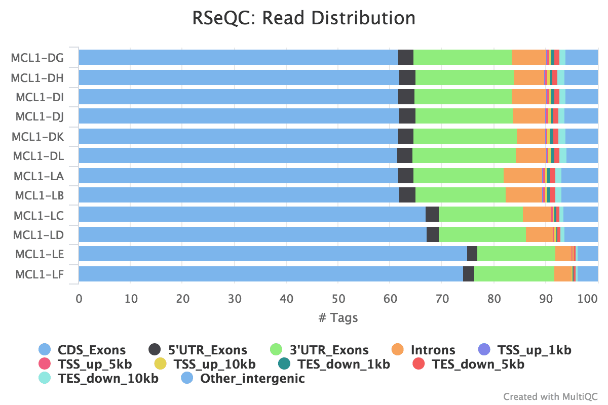
We can also bank check the distribution of reads across known gene features, such as exons (CDS, 5'UTR, 3'UTR), introns and intergenic regions. In RNA-seq we expect most reads to map to exons rather than introns or intergenic regions. It is also the reads mapped to exons that will be counted so it is good to check what proportions of reads have mapped to those. High numbers of readsmapping to intergenic regions could bespeak the presence of Dna contagion.
hands_on Hands-on: Cheque distribution of reads with Read Distribution
Read Distributiontool with the post-obit parameters:
param-collection"Input .bam/.sam file": aligned reads (BAM) (output of HISAT2tool)
param-select"Which tool was used generate logs?": RSeQC
param-select"Type of RSeQC output?": read_distribution
param-collection"RSeQC read_distribution output": Read Distribution output (output of Read Distributiontool)
Audit the Webpage output from MultiQC
The MultiQC plot below shows the result from the full dataset for comparison.
Figure 24: Read Distribution
question Questions
What practice you lot recall of the read distribution?
solution Solution
It looks good, nigh of the reads have mapped to exons and not many to introns or intergenic regions. The samples have pretty consequent read distribution, albeit with slightly higher numbers of readsmapping to CDS exons for MCL1-LC and MCL1-LD, and MCL1-LE and MCL1-LF have more than readsmapping to CDS exons than the other samples.
The MultiQC report can be downloaded past clicking on the floppy deejay icon on the dataset in the history.
question Questions
Can you think of whatsoever other QCs that could be performed on RNA-seq reads?
solution Solution
The reads could be checked for:
Ribosomal contamination
Contamination with other species e.thousand. bacteria
GC bias of the mapped reads
This is single-end data just paired-finish mapped reads could be checked for fragment size (distance between the read pairs).
Conclusion
In this tutorial we have seen how reads (FASTQ files) can be converted into counts. Nosotros have likewise seen QC steps that can exist performed to aid assess the quality of the information. A follow-on tutorial, RNA-seq counts to genes, shows how to perform differential expression and QC on the counts for this dataset.
Key points
In RNA-seq, reads (FASTQs) are mapped to a reference genome with a spliced aligner (e.g HISAT2, STAR)
The aligned reads (BAMs) can so be converted to counts
Many QC steps can be performed to help check the quality of the data
MultiQC can be used to create a prissy summary report of QC information
The Galaxy Rule-based Uploader, Collections and Workflows can help make analysis more efficient and easier
Frequently Asked Questions
Have questions about this tutorial? Cheque out the tutorial FAQ page or the FAQ page for the Transcriptomics topic to see if your question is listed in that location. If not, please ask your question on the GTN Gitter Channel or the Galaxy Assist Forum
Useful literature
Further data, including links to documentation and original publications, regarding the tools, analysis techniques and the interpretation of results described in this tutorial can be found hither.
References
Marcel, M., 2011 Cutadapt removes adapter sequences from high-throughput sequencing reads. EMBnet.periodical 17: 10–12. http://journal.embnet.org/alphabetize.php/embnetjournal/article/view/200
Wang, L., S. Wang, and Westward. Li, 2012 RSeQC: quality command of RNA-seq experiments. Bioinformatics 28: 2184–2185. https://world wide web.ncbi.nlm.nih.gov/pubmed/22743226
Dobin, A., C. A. Davis, F. Schlesinger, J. Drenkow, C. Zaleski et al., 2013 STAR: ultrafast universal RNA-seq aligner. Bioinformatics 29: 15–21. https://academic.oup.com/bioinformatics/article/29/1/xv/272537
Liao, Y., G. K. Smyth, and W. Shi, 2013 featureCounts: an efficient general purpose program for assigning sequence reads to genomic features. Bioinformatics 30: 923–930. https://academic.oup.com/bioinformatics/commodity/31/ii/166/2366196
Liao, Y., One thousand. K. Smyth, and Due west. Shi, 2013 The Subread aligner: fast, accurate and scalable read mapping past seed-and-vote. Nucleic Acids Inquiry 41: e108–e108. 10.1093/nar/gkt214
Fu, North. Y., A. C. Rios, B. Pal, R. Soetanto, A. T. Fifty. Lun et al., 2015 EGF-mediated induction of Mcl-ane at the switch to lactation is essential for alveolar cell survival. Nature Cell Biology 17: 365–375. x.1038/ncb3117
Kim, D., B. Langmead, and S. 50. Salzberg, 2015 HISAT: a fast spliced aligner with low memory requirements. Nature Methods 12: 357. https://www.nature.com/manufactures/nmeth.3317
Ewels, P., M. Magnusson, S. Lundin, and Thousand. Käller, 2016 MultiQC: summarize analysis results for multiple tools and samples in a single report. Bioinformatics 32: 3047–3048. https://academic.oup.com/bioinformatics/article/32/xix/3047/2196507
Feedback
Did y'all use this material every bit an instructor? Feel gratuitous to give us feedback on how it went. Did you lot utilize this textile as a learner or student? Click the form below to go out feedback.
Citing this Tutorial
Maria Doyle, Belinda Phipson, Harriet Dashnow, 2021 1: RNA-Seq reads to counts (Galaxy Training Materials). https://preparation.galaxyproject.org/grooming-material/topics/transcriptomics/tutorials/rna-seq-reads-to-counts/tutorial.html Online; accessed TODAY
Batut et al., 2018 Community-Driven Data Analysis Training for Biology Cell Systems 10.1016/j.cels.2018.05.012
details BibTeX
@misc{transcriptomics-rna-seq-reads-to-counts, author = "Maria Doyle and Belinda Phipson and Harriet Dashnow", title = "one: RNA-Seq reads to counts (Milky way Training Materials)", year = "2021", month = "11", mean solar day = "18" url = "\url{https://training.galaxyproject.org/grooming-material/topics/transcriptomics/tutorials/rna-seq-reads-to-counts/tutorial.html}", notation = "[Online; accessed TODAY]" } @commodity{Batut_2018, doi = {ten.1016/j.cels.2018.05.012}, url = {https://doi.org/10.1016%2Fj.cels.2018.05.012}, yr = 2018, month = {jun}, publisher = {Elsevier {BV}}, volume = {vi}, number = {vi}, pages = {752--758.e1}, author = {B{\'{east}}r{\'{e}}nice Batut and Saskia Hiltemann and Andrea Bagnacani and Dannon Baker and Vivek Bhardwaj and Clemens Blank and Anthony Bretaudeau and Loraine Brillet-Gu{\'{e}}guen and Martin {\v{C}}ech and John Chilton and Dave Clements and Olivia Doppelt-Azeroual and Anika Erxleben and Mallory Ann Freeberg and Simon Gladman and Youri Hoogstrate and Hans-Rudolf Hotz and Torsten Houwaart and Pratik Jagtap and Delphine Larivi{\`{e}}re and Gildas Le Corguill{\'{due east}} and Thomas Manke and Fabien Mareuil and Fidel Ram{\'{\i}}rez and Devon Ryan and Florian Christoph Sigloch and Nicola Soranzo and Joachim Wolff and Pavankumar Videm and Markus Wolfien and Aisanjiang Wubuli and Dilmurat Yusuf and James Taylor and Rolf Backofen and Anton Nekrutenko and Björn Grüning}, title = {Community-Driven Data Analysis Training for Biology}, journal = {Prison cell Systems} }
Congratulations on successfully completing this tutorial!
Practice you lot desire to extend your cognition? Follow one of our recommended follow-up trainings:

0 Response to "Ngs See Distrubution of Reads Over the Gene"
Postar um comentário